Classification Algorithms

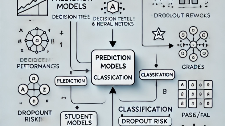
In educational data mining, prediction models play a critical role in analyzing student data to infer specific outcomes, known as predicted variables, from a combination of other features, referred to as predictor variables. These models are applied in various contexts: sometimes to forecast future performance, and at other times to gain insights into current states of learning.

Prediction Models and Classification

One of the most common types of prediction models used in education is classification. Classification models are designed to predict discrete, categorical outcomes. For instance:

• Predicting a student’s grade (e.g., A, B, C, D, or E)
• Identifying a student’s cognitive state (e.g., “Help”, “Confused”, “Doing Well”)
• Determining a binary outcome such as “Pass/Fail” or “True/False”

In the educational domain, these categorical labels can be derived from various sources such as:

• Student records: grades, attendance, or demographic information
• Survey responses: self-reported measures of engagement or motivation
• Learning management systems (LMS): data from student interactions with digital learning platforms
• Instructor coding: manual categorization of student performance or behavior

Example: Student Grade Prediction Using Classification

Consider an example where a classification model is used to predict a student’s final grade in a course. Here, the predicted variable is the student’s grade (A, B, C, D, E), while the predictor variables could include:

• Assignment scores
• Quiz scores
• Time spent on learning resources
• Interaction frequency with online discussion boards
• Attendance in lectures

Classification Techniques in Education

There are several classification algorithms widely used in educational data mining. These include:

1. Logistic Regression: This model is useful when the predicted variable is binary, such as whether a student will pass or fail a course. It models the probability of a certain class (e.g., “Pass” or “Fail”) based on the input features.Example: Predicting whether a student will pass based on their assignment scores and time spent on study materials.
2. Decision Trees: Decision trees are simple, interpretable models that split the data into subsets based on feature values. Each leaf node represents a predicted class.Example: A decision tree could be used to predict whether a student is at risk of dropping out by considering factors such as attendance, assignment submission patterns, and quiz scores.
3. Random Forest: Random Forest is an ensemble learning method that uses multiple decision trees to improve prediction accuracy by averaging their predictions.Example: Predicting a student’s performance level (e.g., high, medium, low) by combining multiple features like class participation, prior grades, and time spent on LMS.
4. XGBoost: A powerful gradient boosting algorithm that builds trees sequentially to reduce prediction errors. It is effective for handling large educational datasets.Example: Predicting student dropouts by considering a combination of academic performance, engagement metrics, and personal attributes.
5. Neural Networks: These are used for more complex, non-linear relationships between predictor variables and categorical outcomes. They require large datasets and are often employed when traditional methods fail to capture intricate patterns.Example: Using neural networks to predict long-term academic success by modeling relationships between various behavioral and performance metrics.

Feature Engineering and Model Selection

In practice, classification models in education rely on well-defined features (i.e., the predictor variables) to make accurate predictions. Feature selection and engineering are critical steps in model building, where data scientists identify the most relevant aspects of student behavior or performance to include in the model.

For example, to predict whether a student will need help (i.e., “Help” vs. “No Help”), relevant features might include:

• Frequency of incorrect quiz submissions
• Time spent reading materials without progressing to the next module
• Infrequent participation in class discussions

An essential consideration when selecting features for a model is to prioritize those with higher construct validity or stronger theoretical grounding. Variables that align well with established theoretical frameworks tend to enhance the model’s generalizability. By leveraging these well-validated features, the resulting models are more likely to perform consistently across different datasets and contexts, improving their robustness and external validity.

Each classification model has strengths and weaknesses depending on the educational context and data complexity. For example, logistic regression is highly interpretable but limited to linear relationships, whereas neural networks are more flexible but less interpretable. Lets dive deeper into some of the classification algorithms:

1. Step Regression (not Stepwise regression) –  is used for binary classification tasks, such as determining whether an outcome is either 0 or 1. While it is less frequently applied on its own today, it serves as the foundational algorithm for many advanced classifiers. Logistic regression models a linear function by selecting input features (parameters), assigning weights to each, and computing the weighted sum of those features to produce a numerical value. The model then applies a predefined threshold, often set at 0.5 (though this can vary), to classify outcomes. If the resulting value is below the threshold, the prediction is assigned as 0; if the value is equal to or above the threshold, the prediction is classified as 1. This simple cutoff mechanism allows logistic regression to distinguish between two classes based on the underlying linear relationship between input features and the outcome.
2. Logistic Regression – is a widely used algorithm for binary classification tasks, where the target variable has only two possible outcomes (e.g., 0/1). It models the relationship between the predictor variables and the outcome by fitting a logistic (sigmoid) function to the data. 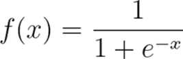The sigmoid function produces an S-shaped curve that maps any real-valued input to a probability between 0 and 1, representing the odds or likelihood of a specific outcome.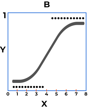One key assumption in logistic regression is that the dependent variable can only take two possible values. This algorithm is particularly effective when interaction effects between features are minimal or not a primary concern, making it a simple yet powerful tool for binary classification.
3. Decision Trees – are particularly effective when modeling variables with interaction effects (or has natural splits), as they inherently capture complex relationships between features by recursively splitting the data based on feature values. Several well-known decision tree classifiers include C4.5 (also known as J48) and CART (Classification and Regression Trees).
   

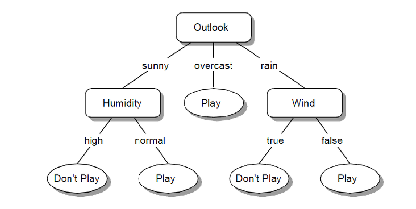
   A simple Decision Tree representing the 2 class problem – Play or Dont-Play

   Decision trees serve as the foundation for more advanced ensemble methods, such as Random Forest and XGBoost, which improve performance by aggregating the outputs of multiple trees. Although individual decision trees are relatively conservative in their predictions, they are more robust to changes in data conditions compared to some other algorithms, making them less sensitive to noise and fluctuations in the dataset. This inherent stability enhances their reliability in dynamic environments.

4. Ensembling is a machine learning approach where multiple models are built and their predictions are combined to improve performance. This can be achieved using techniques like voting, averaging confidence scores, weighted averaging, or by applying a meta-classifier to combine the outputs of different models. Ensembling can take two forms: applying different algorithms to the same dataset (known as stacking) or using the same algorithm on different subsets of the data, with the latter being more common. Tree-based models are particularly popular in ensembling methods.
   

   Types of Ensembling:

   1. Bagging: Involves fitting multiple models (or parameters) in parallel. The models are trained independently on different subsets of the data, and their predictions are combined. An example of this is Random Forest.
   2. Boosting: Involves fitting models sequentially, where each subsequent model tries to correct the errors of the previous ones. This iterative approach helps improve model accuracy by progressively focusing on the harder-to-predict instances.
5. Random Forest is a tree-based ensemble method that uses bagging. It splits the training data into random subsets and, for each subset, selects a random set of features to build a decision tree. The final prediction is made by aggregating the outputs of all the trees through voting. Random Forest is effective with smaller datasets and is relatively interpretable compared to more complex algorithms, as it allows for feature importance extraction to understand which features contribute the most to the model’s predictions.
6. XGBoost, or eXtreme Gradient Boosting, is a tree-boosting algorithm that constructs a series of small trees (typically 4-8 levels) on optimized subsets of the data. The goal of XGBoost is to iteratively build trees that complement one another, progressively improving the fit of the model to the data. It greedily adds new trees, while reducing the impact of earlier trees, and is particularly good at handling both sparse and dense regions of the feature space. XGBoost also incorporates strategies to manage missing or sparse data by learning appropriate default values.Both Random Forest and XGBoost can be applied to regression problems in addition to classification tasks, making them versatile for various types of predictive modeling.

7. Other Methods:

   • Decision Rules: These tend to underfit but are highly interpretable, making them valuable for gaining insights into the data.
   • Support Vector Machines (SVM): SVMs are well-suited for high-dimensional data, as they effectively handle complex relationships between features by finding optimal decision boundaries in multidimensional space.

Ensembling, especially through bagging and boosting, remains a powerful technique to enhance model performance by combining the strengths of individual models.

 

Reference:

Baker, R.S. (2024) Big Data and Education. 8th Edition. Philadelphia, PA: University of Pennsylvania.