
In any classification task, we are predicting a label, which is the categorical outcome we want to forecast, such as whether a student will pass a course. While knowing whether the prediction is correct is important, it is even more valuable to understand how confident the model is in its prediction.
For example, suppose a detector predicts that there is a 50.1% chance that a student will pass a course. Should we celebrate? Not necessarily, because that number alone doesn’t tell us how confident the system is. Confidence matters—a low-confidence prediction might indicate uncertainty, leading us to reconsider interventions.
The Role of Detector Confidence
Detector confidence plays a crucial role in deciding the type and intensity of interventions. Here are three possible interventions based on confidence levels:
- Strong intervention: If the detector confidence is above 60%, take decisive action.
- No intervention: If the confidence is below 40%, it’s not worth intervening.
- Fail-soft intervention: If the confidence is between 40% and 60%, apply a moderate intervention.
These decisions about choosing which intervention(s) can be made using a cost-benefit analysis, which weighs the benefits of a correct intervention against the costs of an incorrect one.
Key Questions in Cost-Benefit Analysis
To guide intervention decisions, we need to ask:
- What is the benefit of a correctly applied intervention? (denoted as aaa)
- What is the cost of an incorrectly applied intervention? (denoted as bbb)
- What is the detector confidence? (denoted as ccc)
The Expected Value of the intervention can be calculated using the formula:
Expected Gain = a*c − b*(1−c)
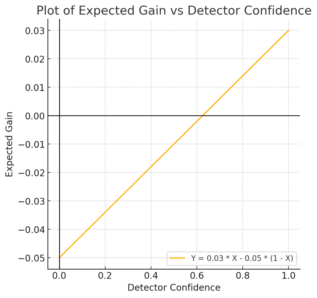
Example Scenario
Let’s consider an educational context where:
- If an intervention is wrongly applied, it costs the student 1 minute.
- Each minute of study helps the student learn 0.05% of the course content.
- A correct intervention helps the student learn 0.03% more content.
Here, a=0.03 and b=0.05. Using the formula:
The Expected value of the intervention is : Expected Gain = 0.03 * confidence – 0.05 (1 – confidence)
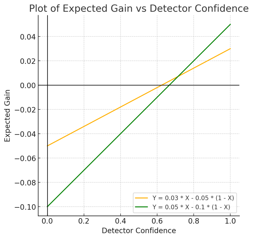
Comparing Two Interventions
Now, imagine a second, stronger intervention. If correctly applied, it offers a boost of 0.05, but if wrongly applied, it costs 0.1. The Expected Gain for this second intervention is similar but the stakes are higher.
From the visual analysis, we can see:
- The first intervention (orange) is effective when detector confidence exceeds 0.62.
- The second, stronger intervention (green) becomes more effective when confidence exceeds 0.71.
Between 0.62 and 0.71, the first intervention is preferable—this is called the “fail-soft range”, where the first intervention is safer and more beneficial.
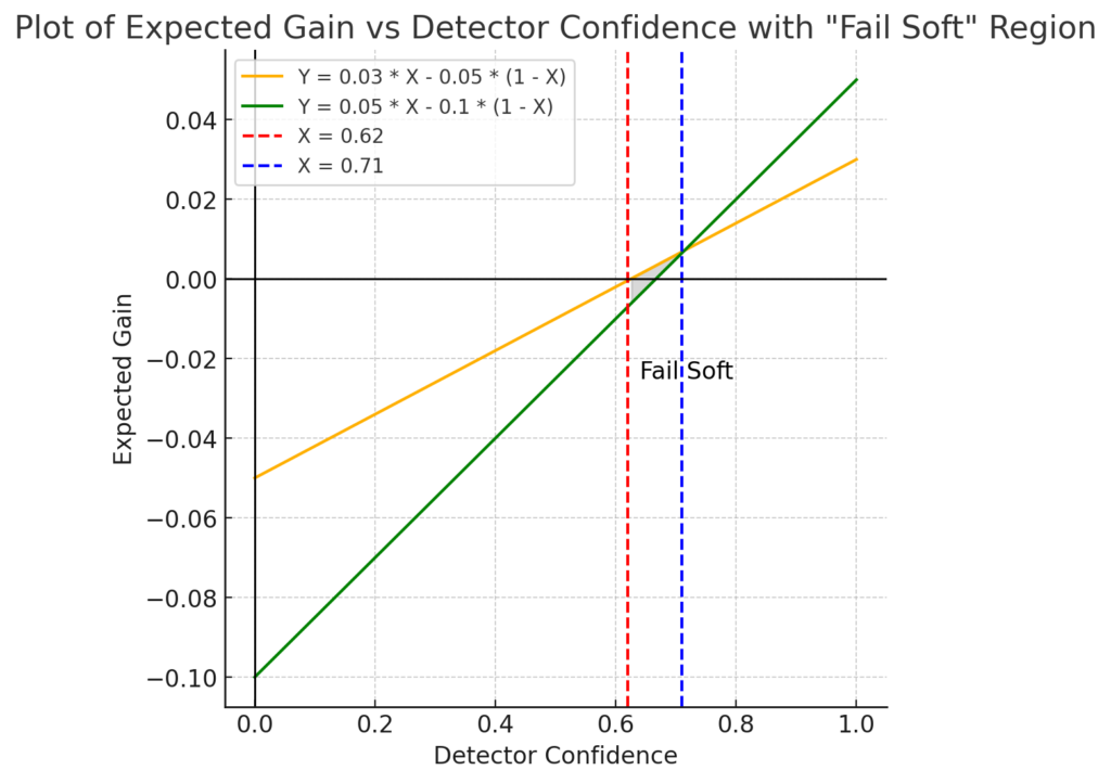
By conducting a cost-benefit analysis, you can determine the most appropriate type of intervention based on the situation. One key insight is that a 50% detector confidence level is not oftent the right threshold for making a decision.
Cost-Sensitive Classification
In addition to analysing interventions based on confidence, cost-sensitive classification can be another approach. Here, false positives (FP) and false negatives (FN) are assigned different costs, rather than treating all errors equally. For instance, fitting a model to minimize an adjusted Root Mean Square Error (RMSE) that weights FP and FN differently can help fine-tune predictions to reflect real-world consequences.
Discovery and Model Analysis
When using AI models for decision-making, retaining the uncertainty of predictions is often crucial. Instead of transforming uncertain predictions into seemingly certain ones, it’s important to maintain the information on confidence levels. This allows us to make more nuanced decisions, especially in educational settings where certainty is rarely absolute. We will discuss about this in another blog post.
Confidence Can Be “Lumpy”
A common issue, especially in earlier models like decision trees, is the lumpiness of confidence. For example, a decision tree might only produce confidence values of 100%, 66.67%, or 50%. This lumpiness is not a flaw, but it can cause certain metrics (like AUC ROC) to behave in unexpected ways, complicating model evaluation.
Leveraging Confidence Intervals
Newer techniques allow us to estimate not only confidence but also the variance or standard deviation around the confidence value. Knowing that a prediction has, for example, 75% confidence with a certain degree of uncertainty is more informative than just the confidence value.
Risk Ratio: Understanding Predictor Impact
Another useful tool in analyzing AI models is the risk ratio, particularly for binary predictors. The formula for the risk ratio (RR) is:
[math] RR = \frac{\text{Probability when predictor } P = 1}{\text{Probability when predictor } P = 0} [/math]
For example, if students who miss 60% of lectures have a 20% chance of failing, and students who attend more than 60% of lectures have only a 5% chance, the risk ratio is:
[math] RR = \frac{0.20}{0.05} = 4 [/math]
This means students who miss more than 60% of lectures are four times more likely to fail, providing clear, interpretable insights into predictor effects.
Tip: You can convert numerical predictors into binary ones using a threshold (as shown in the previous example). This makes it easier to clearly convey the impact of that variable on the predicted outcome.
Conclusion: The Importance of Confidence
In any classification task, understanding and utilizing confidence is critical. Whether applying cost-sensitive classification or analyzing interventions, confidence plays a key role in shaping decisions. By using confidence values effectively and considering metrics like the risk ratio, we can optimize educational interventions and justify our decisions.
Reference:
Baker, R.S. (2024) Big Data and Education. 8th Edition. Philadelphia, PA: Universiwty of Pennsylvania.


